Regression Discontinuity Design (1/2): Theory and Intuition

You’re an avid data scientist and experimenter. You know that randomisation is the summit of Mount Evidence Credibility, and you also know that when you can’t randomise, you resort to observational data and Causal Inference techniques. At your disposal are various methods for spinning up a control group — difference-in-differences, inverse propensity score weighting, and others. With an assumption here or there (some shakier than others), you estimate the causal effect and drive decision-making. But if you thought it couldn’t get more exciting than “vanilla” causal inference, read on.

Personally, I’ve often found myself in at least two scenarios where “just doing causal inference” wasn’t straightforward. The common denominator in these two scenarios? A missing control group — at first glance, that is.

First, the cold-start scenario: the company wants to break into an uncharted opportunity space. Often there is no experimental data to learn from, nor has there been any change (read: “exogenous shock”), from the business or product side, to leverage in the more common causal inference frameworks like difference-in-differences (and other cousins in the pre-post paradigm).

Second, the unfeasible randomisation scenario: the organisation is perfectly intentional about testing an idea, but randomisation is not feasible—or not even wanted. Even emulating a natural experiment might be constrained legally, technically, or commercially (especially when it’s about pricing), or when interference bias arises in the marketplace.

These situations open up the space for a “different” type of causal inference. Although the method we’ll focus on here is not the only one suited for the job, I’d love for you to tag along in this deep dive into Regression Discontinuity Design (RDD).

In this post, I’ll give you a crisp view of how and why RDD works. Inevitably, this will involve a bit of math — a pleasant sight for some — but I’ll do my best to keep it accessible with classic examples from the literature.

In Part 2, we’ll put the theory to work on a real marketplace problem: the impact of listing position on listing performance. But first, let’s build the foundation. Grab yourself a cup of coffee and let’s jump in!

How and why RDD works

Regression Discontinuity Design exploits cutoffs — thresholds — to recover the effect of a treatment on an outcome. More precisely, it looks for a sharp change in the probability of treatment assignment on a ‘running’ variable. If treatment assignment depends solely on the running variable, and the cutoff is arbitrary, i.e. exogenous, then we can treat the units around it as randomly assigned. The difference in outcomes just above and below the cutoff gives us the causal effect.

For example, a scholarship awarded only to students scoring above 90, creates a cutoff based on test scores. That the cutoff is 90 is arbitrary — it could have been 80 for that matter; the line had just to be drawn somewhere. Moreover, scoring 91 vs. 89 makes the whole difference as for the treatment: either you get it or not. But regarding capability, the two groups of students that scored 91 and 89 are not really different, are they? And those who scored 89.9 versus 90.1 — if you insist?

Making the cutoff could come down to randomness, when it’s just a bout a few points. Maybe the student drank too much coffee right before the test — or too little. Maybe they got bad news the night before, were thrown off by the weather, or anxiety hit at the worst possible moment. It’s this randomness that makes the cutoff so instrumental in RDD.

Without a cutoff, you don’t have an RDD — just a scatterplot and a dream. But, the cutoff by itself is not equipped with all it takes to identify the causal effect. Why it works hinges on one core identification assumption: continuity.

The continuity assumption, and parallel worlds

If the cutoff is the cornerstone of the technique, then its importance comes entirely from the continuity assumption. The idea is a simple, counterfactual one: had there been no treatment, then there would’ve been no effect.

To ground the idea of continuity, let’s jump straight into a classic example from public health: does legal alcohol access increase mortality?

Imagine two worlds where everyone and everything is the same. Except for one thing: a law that sets the minimum legal drinking age at 18 years (we’re in Europe, folks).

In the world with the law (the factual world), we’d expect alcohol consumption to jump right after age 18. Alcohol-related deaths should jump too, if there is a link.

Now, take the counterfactual world where there is no such law; there should be no such jump. Alcohol consumption and mortality would likely follow a smooth trend across age groups.

Now, that’s a good thing for identifying the causal effect; the absence of a jump in deaths in the counterfactual world is the necessary condition to interpret a jump in the factual world as the impact of the law.

Put simply: if there is no treatment, there shouldn’t be a jump in deaths. If there is, then something other than our treatment is causing it, and the RDD is not valid.

Two parallel worlds. From left to right; one where there is no minimum age to consume alcohol legally, and one where there is: 18 years.

The continuity assumption can be written in the potential outcomes framework as:

\begin{equation} \lim_{x \to c^-} \mathbb{E}[Y_i(0) \mid X_i = x] = \lim_{x \to c^+} \mathbb{E}[Y_i(0) \mid X_i = x] \label{eq: continuity_po}
\end{equation}

Where $Y_i(0)$ is the potential outcome, say, risk of death of subject $\mathbb{i}$ under no treatment.

Notice that the right-hand side is a quantity of the counterfactual world; not one that can be observed in the factual world, where subjects are treated if they fall above the cutoff.

Unfortunately for us, we only have access to the factual world, so the assumption cannot be tested directly. But, luckily, we can proxy it. We will see placebo groups achieve this in Part 2. But first, we start by identifying what can break the assumption:

1. Confounders: something other than the treatment happens at the cutoff that also impacts the outcome. For instance, adolescents resorting to alcohol to alleviate the crushing pressure of being an adult now — something that has nothing to do with the law on the minimum age to consume alcohol (in the no-law world), but that does confound the effect we are after, happening at the same age — the cutoff, that is.
2. Manipulating the running variable: When units can influence their position with regard to the cutoff, it may be that units who did so are inherently different from those who did not. Hence, cutoff manipulation can result in selection bias: a form of confounding. Especially if treatment assignment is binding, subjects may try their best to get one version of the treatment over the other.

Hopefully, it’s clear what constitutes a RDD: the running variable, the cutoff, and most importantly, reasonable grounds to defend that continuity holds. With that, you’ve gotten yourself a neat and effective causal inference design for questions that can’t be answered by an A/B test, nor by some of the more common causal inference techniques like diff-in-diff, nor with stratification.

In the next section, we continue shaping our understanding of how RDD works; how does RDD “control” confounding relationships? What exactly does it estimate? Can we not just control for the running variable too? These are questions that we tackle next.

RDD and instruments

If you are already familiar with instrumental variables (IV), you may see the similarities: both RDD and IV leverage an exogenous variable that does not cause the outcome directly, but does influence the treatment assignment, which in turn may influence the outcome. In IV this is a third variable Z; in RDD it’s the running variable that serves as an instrument.

Wait. A third variable; maybe. But an exogenous one? That’s less clear.

In our example of alcohol consumption, it is not hard to imagine that age — the running variable — is a confounder. As age increases, so might tolerance for alcohol, and with it the level of consumption. That’s a stretch, maybe, but not implausible.

Since treatment (legal minimum age) depends on age — only units above 18 are treated — treated and untreated units are inherently different. If age also influences the outcome, through a mechanism like the one sketched above, we got ourselves an apex confounder.

Still, the running variable plays a key role. To understand why, we need to look at how RDD and instruments leverage the frontdoor criterion to identify causal effects.

Backdoor vs. frontdoor

Perhaps almost instinctively, one may answer with controlling for the running variable; that’s what stratification taught us. The running variable is confounder, so we include it in our regression, and close the backdoor. But doing so would cause some trouble.

Remember, treatment assignment depends on the running variable so that everyone above the cutoff is treated with all certainty, and certainly not below it. So, if we control for the running variable, we run into two very related problems:

1. Violation of the Positivity assumption: this assumption says that treated units should have a non-zero probability to receive the opposite treatment, and vice versa. Intuitively, conditioning on the running variable is like saying: “Let’s estimate the effect of being above the minimum age for alcohol consumption, while holding age fixed at 14.” That does not make sense. At any given value of running variable, treatment is either always 1 or always 0. So, there’s no variation in treatment conditional on the running variable to support such a question.
2. Perfect collinearity at the cutoff: in estimating the treatment effect, the model has no way to separate the effect of crossing the cutoff from the effect of being at a particular value of X. The result? No estimate, or a forcefully dropped variable from the model design matrix. Singular design matrix, does not have full rank, these should sound familiar to most practitioners.

So no — conditioning on the running variable doesn’t make the running variable the exogenous instrument that we’re after. Instead, the running variable becomes exogenous by pushing it to the limit—quite literally. There where the running variable approaches the cutoff from either side, the units are the same with respect to the running variable. Yet, falling just above or below makes the difference as for getting treated or not. This makes the running variable a valid instrument, if treatment assignment is the only thing that happens at the cutoff. Judea Pearl refers to instruments as meeting the front-door criterion.

In this post I try to bridge RDD and IV perhaps more than is warranted. Conventionally, fuzzy RDD has been framed as a form of IV, but sharp RDD hasn’t been so. Instead, sharp RDD identification relies on the assumed as-random property of the units around the cutoff. Take the above explanation to build intuition, but beware that it is arbitrary.

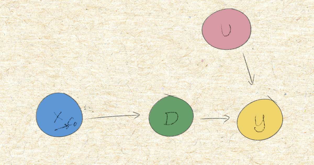X is the running variable, D the treatment assignment, Y the outcome, and U is a set of unobserved influences on the outcome. The causal effect of D on Y is unidentified in the above marginal model, for X being a confounder, and U potentially too. Conditioning on X violates the positivity assumption. Instead, conditioning X on its limits towards cutoff (c0), controls for the backdoor path: X to Y directly, and through U.

LATE, not ATE

So, in essence, we’re controlling for the running variable — but only near the cutoff. That’s why RDD identifies the local average treatment effect (LATE), a special flavour of the average treatment effect (ATE). The LATE looks like:

\begin{equation} \delta_{SRD}=E\big[Y^1_i – Y_i^0\mid X_i=c_0] \end{equation}

The local bit refers to the partial scope of the population we are estimating the ATE for, which is the subpopulation around the cutoff. In fact, the further away the data point is from the cutoff, the more the running variable acts as a confounder, working against the RDD instead of in its favour.

Back to the context of the minimum age for legal alcohol consumption example. Adolescents who are 17 years and 11 months old are really not so different from those that are 18 years and 1 month old, on average. If anything, a month or two difference in age is not going to be what sets them apart. Isn’t that the essence of conditioning on, or holding a variable constant? What sets them apart is that the latter group can consume alcohol legally for being above the cutoff, and not the former.

This setup enables us to estimate the LATE for the units around the cutoff and with that, the effect of the minimum age policy on alcohol-related deaths.

We’ve seen how the continuity assumption has to hold to make the cutoff an interesting point along the running variable in identifying the causal effect of a treatment on the outcome. Namely, by letting the jump in the outcome variable be entirely attributable to the treatment. If continuity holds, the treatment is as-good-as-random near the cutoff, allowing us to estimate the local average treatment effect.

In Part 2, we’ll walk through exactly that: a real-world RDD estimating the causal effect of search ranking position on listing performance in an online marketplace. We’ll cover the practical setup, modelling choices, placebo testing, and density checks.

Wrapping up

We’ve covered the conceptual core of RDD: the continuity assumption and why it matters, how the running variable acts as an instrument near the cutoff, the front-door identification logic, and what makes the LATE a valid (but local) causal estimate. These are the building blocks you need before running any RDD in practice.

Ready to see it applied? Head over to Part 2: RDD in Action.

If you want to read more broadly, here are some resources:

• Causal Inference Mixtape: for an extensive read on RDD and more
• Causal Inference: A Statistical Learning Approach: formal and technically to the point
• and of course our trusty Wikipedia (actually great to get started)

You can stay up to date with my writing by following me on Medium, or just visiting here often 👍